The Stark Realities of Reproducible Sociological Research
Alternative titles: Some Newer Rules of the Sociological Method or The Moon Under Water
Professor Vernon Gayle, University of Edinburgh, UK.
Please remember that this work is very exploratory.
Positive comments are always appreciated, but brickbats improve work.
Here is how to contact me
Table of Contents:
Notebook Meta Information
Computing Environment and Software
Research Meta Information
Data Description
Data Enabling
Data Analysis
- Duplicating the Connolly (2006) Model Results in R
- Duplicating the Connolly (2006) Model Results in SPSS
- Duplicating the Connolly (2006) Model Results in Stata
- Duplicating the Connolly (2006) Model Results in Python
- Replicating the Connolly (2006) Model Results Adding Quasi-Variance
- Replicating the Connolly (2006) Model Results Adding NS-SEC
Data Documentation
Commentary
Notes
License 
This work must not be copied or cited without written permision from the author
Copyright (c) 2017 Vernon Gayle, University of Edinburgh
When the work is nearer completion I will make it more open with an
The MIT License (MIT)
which will say...
Copyright (c) 2017 Vernon Gayle, University of Edinburgh
Permission is hereby granted, free of charge, to any person obtaining a copy of this software and associated documentation files (the "Software"), to deal in the Software without restriction, including without limitation the rights to use, copy, modify, merge, publish, distribute, sublicense, and/or sell copies of the Software, and to permit persons to whom the Software is furnished to do so, subject to the following conditions:
The above copyright notice and this permission notice shall be included in all copies or substantial portions of the Software.
THE SOFTWARE IS PROVIDED "AS IS", WITHOUT WARRANTY OF ANY KIND, EXPRESS OR IMPLIED, INCLUDING BUT NOT LIMITED TO THE WARRANTIES OF MERCHANTABILITY, FITNESS FOR A PARTICULAR PURPOSE AND NONINFRINGEMENT. IN NO EVENT SHALL THE AUTHORS OR COPYRIGHT HOLDERS BE LIABLE FOR ANY CLAIM, DAMAGES OR OTHER LIABILITY, WHETHER IN AN ACTION OF CONTRACT, TORT OR OTHERWISE, ARISING FROM, OUT OF OR IN CONNECTION WITH THE SOFTWARE OR THE USE OR OTHER DEALINGS IN THE SOFTWARE.
Authorship and Meta Information 
Author: Professor Vernon Gayle Orcid id: http://orcid.org/0000-0002-1929-5983
Project: Reproducible Sociological Research
Sub-project: Stratification Conference (Edinburgh) September 2017
Using this Notebook 
Using Jupyter notebooks for large-scale social science data analysis in sociology is zygotic.
This is an early example of undertaking a complete analytical workflow within a Jupyter notebook.
As this practice becomes more ubiquitos it is likely that there will be improvements and best practices will become much more evident.
Warning.
Within this Jupyter notebook there has been a lot of non-routine work. For example I have 'swivel-chaired' between data analytical software packages and changed kernels.
It may from time to time be necessary to re-start the notebook depending on how stable your computing environment is.
Therefore in some sections I re-start a R session.
Please remember that this work is very exploratory.
Positive comments are always appreciated, but brickbats improve work.
Here is how to contact me
Updates 
Latest Update: 28th June (pushed up to https://github.com/vernongayle/new_rules_of_the_sociological_method ) and e-mailed to colleagues.
Previous Updates:
27th June (my Mum's birthday) General work 26th June Ethics Approval Form Submitted 25th June Pre-paratory work begins 24th June Pre-Analysis Plan submitted to date stamping
Pre-Analysis Plan 
A pre-analysis plan is openly available (in word format) https://github.com/vernongayle/new_rules_of_the_sociological_method/blob/master/pre_analysis_plan_20170624_vg_v1.docx .
The pre-analysis plan has been formally timestamped by Originstamp.
hash: ca0fc7d948fd67cf8a1a2ac9111e9bf40425c010dfdf76ef33a0e578a90981a8
Submitted to OriginStamp: 24 Jun 2017 21:00:24 GMT Submitted to the Blockchain: 25 Jun 2017 16:00:21 GMT
This document can be verifyied using the hash at https://app.originstamp.org/verify .
Note: Some researcher might not consider this document to be a pure pre-analysis plan. This is because I have examined the data and worked with it previously. However, it is an example of how a pre-analysis plan could work in the sociological analysis of an existing large-scale social survey dataset.
Research Ethics Approval Application 
A research ethics approval application has been made to the School of Social and Political Science, University of Edinburgh https://github.com/vernongayle/new_rules_of_the_sociological_method/blob/master/Research_Ethics_Form_20170626_vg_v1.pdf .
Research Ethics Approval 
From: MOORE Niamh
Sent: 26 June 2017 17:01
To: GAYLE Vernon
Hi Vernon,
Approved at level 1. If only they were all so straightforward.
Good luck with the project.
All the best
Niamh
All the best with your application.
Niamh
Dr Niamh Moore
Chancellor's Fellow I Deputy Director of Research (Ethics)
Sociology I Room 3.09, 3F2 I 18 Buccleuch Place
School of Social and Political Sciences I University of Edinburgh I Edinburgh EH8 8LN
niamh.moore@ed.ac.uk l @rawfeminism l +44(0)131-6508260 l skype: niamhresearcher http://www.sociology.ed.ac.uk/people/staff/niamh_moore
Overview of the Reproducibility Checklist
http://www.bitss.org/2015/12/31/science-is-show-me-not-trust-me/
Philip Stark outlines 14 reproducibility points that an analysis can fail on
- If you relied on Microsoft Excel for computations, fail.
- If you did not script your analysis, including data cleaning and munging, fail.
- If you did not document your code so that others can read and understand it, fail.
- If you did not record and report the versions of the software you used (including library dependencies), fail.
- If you did not write tests for your code, fail.
- If you did not check the code coverage of your tests, fail.
- If you used proprietary software that does not have an open-source equivalent without a really good reason, fail.
- If you did not report all the analyses you tried (transformations, tests, selections of variables, models, etc.) before arriving at the one you chose to emphasize, fail.
- If you did not make your code (including tests) available, fail.
- If you did not make your data available (and a law like FERPA or HIPPA doesn’t prevent it), fail.
- If you did not record and report the data format, fail.
- If there is no open source tool for reading data in that format, fail.
- If you did not provide an adequate data dictionary, fail.
- If you published in a journal with a paywall and no open-access policy, fail.
Literate Computing
Fernando Perez says
"Literate Computing is the weaving of a narrative directly into a live computation, interleaving text with code and results to construct a complete piece that relies equally on the textual explanations and the computational components, for the goals of communicating results in scientific computing and data analysis" (see http://blog.fperez.org/).
Literate programming is a paradigm introduced by Donald Knuth in which a program is given as an explanation of its logic in a human readable language (e.g. plain English) with snippets traditional source code (or macros) (see https://en.wikipedia.org/wiki/Literate_programming).
A challenge of this current sub-project is simple - can I undertake a plausible piece of analysis, using genuine large-scale data with realistic levels of messiness, that is 'literate' as well as reproducible?
Computing Environment and Software
Computing Environment
Work undertaken using machine surface pro 109.152.252.166 (my public IP address).
Processor: Intel(R) Core™ i5-4300U CPU@ 1.90 GHz 2.50 GHz
Installed memory (RAM): 4.00 GB
System type: 64-bit Operating System, x-64 based processor
WARNING
You must have R installed on your machine.
You must have installed the R kernel (See https://anaconda.org/r/r-irkernel ).
You must have installed the R libraries foreign and survey
for example run the code install.packages("foreign","survey")
(see https://cran.r-project.org/web/packages/survey/index.html ; https://cran.r-project.org/web/packages/foreign/index.html).
Reminder *Switch Kernel to R < Menu kernel - change kernel>*
Getting the libraries for R
library(foreign)
library(survey)
library(car)
library(dplyr)
library(weights)
library(dummies)
Various WARNINGS will appear. Don't panic.
If you have a more serious ERROR message here it is possibly because you have not switched to the _R Kernel_.
The Code Test 
Part 1 Logistic Regression
In this block of the work I undertake a test of the software.
Because the analyses below will be based on a logistic regression model I have chosen to check the results of a logit model in my software environment against a known result.
In this section I will import a dataset from the Stata website (www.stata-press.com) and estimate a logit model.
myautodata <- read.dta("http://www.stata-press.com/data/r12/auto.dta")
summary(myautodata)
Estimating a logistic regression model.
- Outcome variable = foreign
- Explanatory variables = weight + mpg
myautologit1 <- glm(foreign ~ weight + mpg, data = myautodata, family = "binomial")
Summarizing the output of the logistic regression model.
summary(myautologit1)
These results are identical to the results that are found in the Stata Manual p.1271.
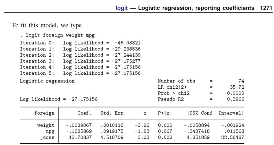
Therefore I am confident that the software environment is providing the correct results for a logistic regression model.
Because I intend to use quasi-variances I will also test analyses below will be based on a logistic regression model I have chosen to check the results of a logit model in my software environment against a known result.
In this section I will import a dataset from the Stata website (www.stata-press.com) and estimate a logit model.
Part II Quasi-Variance Estimation
In the replication part of the analysis I intend to calculate quasi-variance estimates after estimating the logistic regression model. As a furth code test I will use the ship damage data and estimate an overdispersed poisson loglinear model for ship damage data from McCullagh and Nelder (1989), Sec 6.3.2.
_Make sure that in R qvcalc is installed_
code required in R
install.packages('qvcalc')
library(MASS)
library(qvcalc)
data(ships)
ships$year <- as.factor(ships$year)
ships$period <- as.factor(ships$period)
shipmodel <- glm(formula = incidents ~ type + year + period,
    family = quasipoisson,
    data = ships, subset = (service > 0), offset = log(service))
summary(shipmodel)
shiptype.qvs <- qvcalc(shipmodel, "type")
summary(shiptype.qvs, digits = 4)
plot(shiptype.qvs)
These results are identical to the results that are found in Firth, D. and De Menezes, R.X., 2004. Quasi-variances. Biometrika, pp.65-80.
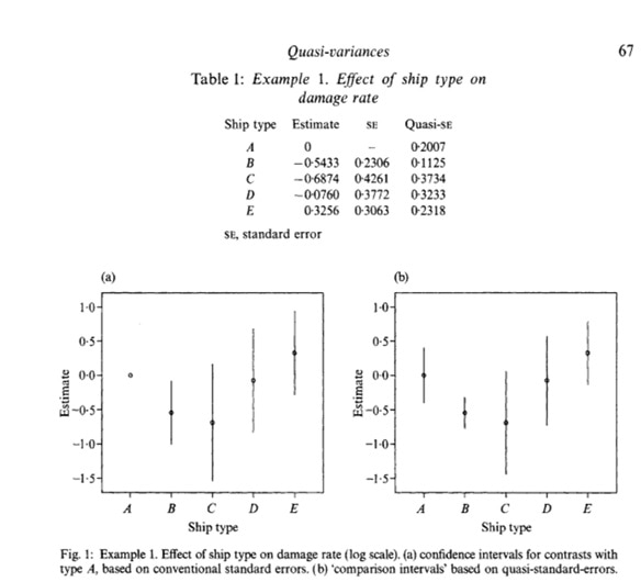
Therefore I am confident that the software environment is providing the correct results for quasi-variance estimates.
The Research Dataset 
The Youth Cohort Study of England and Wales (YCS)
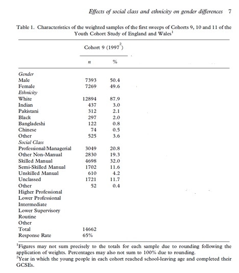
The Youth Cohort Study of England and Wales (YCS) is a major longitudinal study that began in the mid-1980s. It is a large-scale nationally representative survey funded by the government and is designed to monitor the behaviour of young people as they reach the minimum school leaving age and either remain in education or enter the labour market.
There are a number of challenges associated with analysing YCS data, most notably inadequate documentation of the procedures used to construct the data-sets.
YCS Cohort Nine (1998-2000) UK Data Archive Study 4009
https://discover.ukdataservice.ac.uk/catalogue/?sn=4009
The population studied was male and female school pupils in England and Wales who had reached minimum school leaving age in the 1996/1997 school year. To be eligible for inclusion they had to be aged 16 on August 31st 1997.
Downloaded: UK Data Service https://www.ukdataservice.ac.uk/
Date: 19th June 2017
Time: 19:54
Finch, S.A., La Valle, I., McAleese, I., Russell, N., Nice, D., Fitzgerald, R., Finch, S.A. (2004). Youth Cohort Study of England and Wales, 1998-2000. [data collection]. 5th Edition. UK Data Service. SN: 4009, http://doi.org/10.5255/UKDA-SN-4009-1
Data Enabling (a real attempt with the raw data)
Description of the dataset
The dataset used in this set of analyses is from YCS cohort 9 - sweep 1.
The file is called "ycs9sw1".
The file will be read in Stata format (i.e. th ycs9sw1.dta).
Data Wrangling (a real attempt with the raw data) 
# If you have not run the notebook sequentially...

# theses libraries are required

library(foreign)
library(survey)
library(car)
library(dplyr)
library(weights)
library(dummies)
Various WARNINGS will appear. Don't panic!
This file is located on (my) OneDrive.
An internet connection is useful but it is not required, as the dataset is stored locally.
When reading your version of the data from your specific location....
Remember that C:/temp/ (is windows) is C:/data/ here in the Jupyter notebook.
# This file is located on (my) OneDrive.

mydata.df <- read.dta("C:/Users/Vernon/OneDrive - University of Edinburgh/Documents/ycs_9_2017/UKDA-4009-stata8/stata8/ycs9sw1.dta")
Various WARNINGS will appear. Don't panic!
These error messages occur because R is reading a Stata .dta file. It is a genuine large-scale research dataset and includes a large number of value labels and variable labels.
summary(mydata.df)
Various WARNINGS will appear. Don't panic.
To see the summary of the data use the scroll bar to scroll down.
Get a subset of the data with only the variables needed.
myvars <- c("serial", "weight", "sex", "s1a_c", "a58", "s1eth", "s1acqe", "pseg", "pseg1", "pseg2", "pseg3", "pseg4", "pseg5", "pseg6", "pseg7")
mydata.df <- mydata.df[myvars]
summary(mydata.df)
str compactly display the internal structure of an R object.
It is a diagnostic function and an alternative to summary.
str(mydata.df)
View the data in spreadsheet format.
head(mydata.df)
Construct the outcome variable
The binary indicator of 5+ GCSEs A (star) - C will be "s15a_c" .
It is constructed from variable "s1a_c" - the number of GCSEs A (star) - C.
Tabulate the original outcome "s1a_c" number of GCSEs A (star) - C .
table(mydata.df$s1a_c)
Construct the binary outcome variable "s15a_c" 5+ GCSEs at grades A-C
Following the existing naming convention used in YCS Cohort 9 I have chosen the title "s15a_c" because this is a sweep 1 measure "s1" of 5+ GCSEs at grades A-C "5a_c" hence "s15a_c".
Create the "empty" new field.
mydata.df$s15a_c <- NA
table(mydata.df$s15a_c)
The new field "$s15a_c" is empty.
Recode the old field into the new one for the specified rows.
mydata.df$s15a_c[mydata.df$s1a_c>4] <-1
table(mydata.df$s15a_c)

mydata.df$s15a_c[mydata.df$s1a_c<5] <-0
table(mydata.df$s15a_c)
Construct the first variable explanatory variable girls (gender)
The binary indicator of girls (gender) from the existing variable "sex" .
This is a factor. Therefore I will check levels in the original data boys==1 and girls==2.
levels(mydata.df$sex)
table (mydata.df$sex)
Create the "empty" new field.
# create the new field
mydata.df$girls <- NA
table(mydata.df$girls)
The new field "$girls" is empty.
Recode the old field into the new one for the specified rows.
mydata.df$girls[mydata.df$sex=="male"] <-0
mydata.df$girls[mydata.df$sex=="female"] <-1
table(mydata.df$girls)
Construct the explanatory variable for ethnicity
Beware this measure is messy!
This is a factor. Therefore I check levels in the original data.
levels(mydata.df$a58)
Now I create a table of the ethnicity measure "a58".
table(mydata.df$a58)
These are the dummies that are required for the model in Connolly (2006, p.20)
Chinese
Indian
White
Bangladeshi
Pakistani
Strangely, the "Other" category is not in the model!
Ethnic categories required for the analysis.
These are the categories developed and used in Connolly (2006) Table 1 (p.7)
White Indian Pakistani Black Bangladeshi Chinese Other
Here are the labels and codes in the YCS dataset
- 1 "white"
- 2 "carib." "afro." "other black"
- 3 "indian"
- 4 "pakistani"
- 5 "bangladeshi"
- 6 "chin!ese"
- 7 "other asian"
- 10 "any other"
- 97 "mixed ethnic origin"
- . "ref!used"
Here are my estimates of the number is each ethnic category used in Connolly (2006) Table 1 (p.7)
1 White 12993
2 Black 260
3 Indian 436
4 Pakistani 280
5 Bangladeshi 112
6 Chinese 78
7 Other 503
Create the new field "ethnic1".
Everyone is placed into category 7.
I then recode the new field "ethnic1" with values from "a58" .
There is an explanation of this unorthodox approach below...
# create the new field,

mydata.df$ethnic1 <- 7

# everyone is placed into category 7.

# recode the new field with values from the old field.
mydata.df$ethnic1[mydata.df$a58=="white"] <-1
mydata.df$ethnic1[mydata.df$a58=="carib."] <-2
mydata.df$ethnic1[mydata.df$a58=="afro."] <-2
mydata.df$ethnic1[mydata.df$a58=="other black"] <-2
mydata.df$ethnic1[mydata.df$a58=="indian"] <-3
mydata.df$ethnic1[mydata.df$a58=="pakistani"] <-4
mydata.df$ethnic1[mydata.df$a58=="bangladeshi"] <-5
mydata.df$ethnic1[mydata.df$a58=="chin!ese"] <-6
mydata.df$ethnic1[mydata.df$a58=="other asian"] <-7
mydata.df$ethnic1[mydata.df$a58=="any other"] <-7
mydata.df$ethnic1[mydata.df$a58=="mixed ethnic origin"] <-7
mydata.df$ethnic1[mydata.df$a58=="ref!used"] <-7
There appears to be a quirk in the labelling of the missing values "." in the Stata file.
I have got around this by forcing these cases into category 7 when I created the new field
i.e. mydata.df$ethnic1 <- 7
Create a table of the new "ethnic1" variable.
table(mydata.df$ethnic1)
This might not be the neatest solution! But the obstactle has been overcome.
# Just to check the variable again.

table(mydata.df$ethnic1)
# Double check ethnic1 is not a factor

levels(mydata.df$ethnic1)
Construct a series of dummy variables for ethnicity
I have chosen to construct a each variable manually, in order to double check it.
White pupils.
mydata.df$white <-0
table(mydata.df$white)
mydata.df$white[mydata.df$ethnic1=="1"] <-1
table(mydata.df$white)
Black pupils.
mydata.df$black <-0
table(mydata.df$black)
mydata.df$black[mydata.df$ethnic1=="2"] <-1
table(mydata.df$black)
Indian pupils
mydata.df$indian <-0
table(mydata.df$indian)
mydata.df$indian[mydata.df$ethnic1=="3"] <-1
table(mydata.df$indian)
Pakistani pupils.
mydata.df$pakistani <-0
table(mydata.df$pakistani)
mydata.df$pakistani[mydata.df$ethnic1=="4"] <-1
table(mydata.df$pakistani)
Bangladeshi pupils.
mydata.df$bangladeshi <-0
table(mydata.df$bangladeshi)
mydata.df$bangladeshi[mydata.df$ethnic1=="5"] <-1
table(mydata.df$bangladeshi)
Chinese pupils.
mydata.df$chinese <-0
table(mydata.df$chinese)
mydata.df$chinese[mydata.df$ethnic1=="6"] <-1
table(mydata.df$chinese)
Other pupils.
mydata.df$other <-0
table(mydata.df$other)
mydata.df$other[mydata.df$ethnic1=="7"] <-1
table(mydata.df$other)
The block of dummy variables representing ethnicity have been constructed.
Now I perform a brief test.
Here is a table of the outcome variable 5+ GCSEs at grades A - C.
table(mydata.df$s15a_c)
Here is a table of ethnicity.
table(mydata.df$ethnic1)
Here is a table of school GCSE outcome by ethnicity
mytable <- table(mydata.df$ethnic1, mydata.df$s15a_c) # A will be rows, B will be columns
mytable # print table
There results look plausible and I am happy that the measures are behaving themselves.
Construct the explanatory variable for social class
Beware this a bit messy!
The variables pseg1 - pseg7 are social class dummies.
I would like these variables to have names that are more "human-eye-readable".
Here is the first social class dummy "pseg1" which is the Professional/Managerial social class.
table(mydata.df$pseg1)
Here we will be using the reshape library.
Make sure that it has been installed make sure that it has been installed
The R code is
install.packages ("reshape")
library(reshape)
Various WARNINGS might appear. Don't panic.
Here is the code to rename "pseg1" as "prof_man" i.e.
mydata.df <- rename(mydata.df, c(pseg1="prof_man"))
Now take a look at the "renamed" variable.
table(mydata.df$prof_man)
I now rename pseg2 - pseg4.
mydata.df <- rename(mydata.df, c(pseg2="o_non_man"))
table(mydata.df$o_non_man)
mydata.df <- rename(mydata.df, c(pseg3="skilled_man"))
table(mydata.df$skilled_man)
mydata.df <- rename(mydata.df, c(pseg4="semi_skilled"))
table(mydata.df$semi_skilled)
The dataset has now been 'wrangled' or 'enabled' and should be in reasonable shape to test.
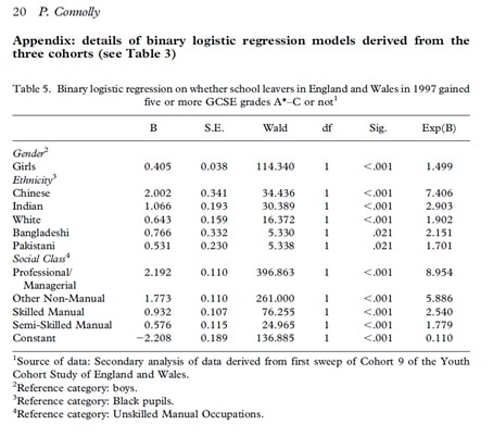
In the next stage I test the data and ultimately I will try to duplicate the model in Connelly (2006, p.20).
Now I save the wrangled data frame in a file called ycs9sw1.rda.
save(mydata.df,file="C:/Users/Vernon/OneDrive - University of Edinburgh/Documents/ycs_9_2017/ycs9sw1.rda")
List the objects in my workspace.
ls()
Now I am going to remove "rm" these objects.
rm ("mydata.df", "mytable", "myvars")
ls()
Data Test 
In this section I undertake a small series of exploratory data analysis tasks to check the data with the published results in Connolly (2006).
Re-loading the data frame from the saved file.
load("C:/Users/Vernon/OneDrive - University of Edinburgh/Documents/ycs_9_2017/ycs9sw1.rda")
ls()
Now I set up the survey desing of the YCS 9.
Within an object called "small.w" I specify the design.
The "ids" are the identification for each case i.e. "serial".
The data are "mydata.df".
The survey weights are "weight".
small.w <- svydesign(ids = ~serial, data = mydata.df, weights = ~weight)
Now I attempt to check the values of my variables against the values (n) and proportions reported in Connolly (2006, p.7, Table 1).
Girls.
table(svytable(~girls, design = small.w))
prop.table(svytable(~girls, design = small.w))
These results are correct. Checked with Connolly (2006, p.7, Table 1).
Ethnicity.
table(svytable(~ethnic1, design = small.w))
prop.table(svytable(~ethnic1, design = small.w))
These results are correct.
Checked with Connolly (2006, p.7, Table 1).
Remember that the ordering in Connolly (2006, p.7, Table 1) is not the same as in the logit model Connolly (2006, p.20).
Social class.
Here I remind myself of the variable names.
I use str which is a compact display of the "structure" of an arbitrary R object.
str(mydata.df)
print("prof_man")
table(svytable(~prof_man , design = small.w))
prop.table(svytable(~prof_man , design = small.w))

print("o_non_man")
table(svytable(~o_non_man , design = small.w))
prop.table(svytable(~o_non_man , design = small.w))

print("skilled_man")
table(svytable(~skilled_man, design = small.w))
prop.table(svytable(~skilled_man , design = small.w))

print("semi_skilled")
table(svytable(~semi_skilled , design = small.w))
prop.table(svytable(~semi_skilled , design = small.w))
These results are correct.
Checked with Connolly (2006, p.7, Table 1).
Remember that the categories used in the logit model Connolly (2006, p.20). are not the same as in Connolly (2006, p.7, Table 1).
In this section I have undertaken a small series of exploratory data analysis tasks to check the data with the published results in Connolly (2006).
I am confident that the data are in good shape ready for duplicating the logit model.
Data Analysis 
Beware if you skipped to this section then make sure that you have the correct data frame (i.e. the data file "ycs9sw1.rda").
Re-loading the data frame from the saved file requries this R code
_load("C:/Users/Vernon/OneDrive - University of Edinburgh/Documents/ycs_92017/ycs9sw1.rda")
ls()
It is currently in the markdown cell below.
You might also require the R libraries.
Setting up the survey design of the YCS data.
library(foreign)
library(survey)
library(car)
library(dplyr)
library(weights)
library(dummies)
load("C:/Users/Vernon/OneDrive - University of Edinburgh/Documents/ycs_9_2017/ycs9sw1.rda")
ls()
mydesign1 <- svydesign(id = ~serial,data = mydata.df, weight = ~weight)
This is a svy (i.e.survey) logit regression model.
The outcome variable is "s15a_c" - 5+ GCSEs at grades A - C .
The explanatory variables are
girls
ethnicity (represented by a block of dummy variables)
social class (represented by a block of dummy variables).
model1<-svyglm (s15a_c ~ girls + chinese + indian +
                 white + bangladeshi + pakistani +
                 pakistani + prof_man + o_non_man +
                 skilled_man + semi_skilled, design=mydesign1, data = mydata.df, family = "binomial")
There might be a warning message because we are modelling survey (i.e. weighted) data.
Don't panic.
Summary of the model results.
summary (model1)
These results are not the same as the results presented in Table 5, p.20 Connolly (2006).
The difference may not be immediately apparent.
In the published work Connelly (2006)
a) the pupils in ethnic category "other" are dropped from the analysis
b) the pupils in class categories "other" and "unclassified" are dropped from the analysis.
Here we subset ethnic categories 1 - 6.
table(mydata.df$ethnic1)
Here we subset ethnic categories 1 - 6.
mydata2.df <- subset(mydata.df, ethnic1!=7)
table(mydata.df$ethnic1)
table(mydata2.df$ethnic1)
Here we subset pupils in class categories pseg1 - pseg5.
table(mydata2.df$pseg6)
table(mydata2.df$pseg7)
mydata3.df <- subset(mydata2.df, pseg6!=1)
table(mydata.df$pseg6)
table(mydata3.df$pseg6)
mydata4.df <- subset(mydata3.df, pseg7!=1)
table(mydata.df$pseg7)
table(mydata4.df$pseg7)
The dataset should be in shape now for estimating the (survey) logit model.
Beware you might need to reset the design.
mydesign2 <- svydesign(id = ~serial,data = mydata4.df, weight = ~weight)
model2<-svyglm (s15a_c ~ girls + chinese + indian +
                 white + bangladeshi + pakistani +
                 pakistani + prof_man + o_non_man +
                 skilled_man + semi_skilled, design=mydesign2, data = mydata4.df, family = "binomial")
There might be a warning message because we are modelling survey (i.e. weighted) data.
Don't panic.
Summary of the model results.
summary (model2)
These results are now the same as in the published model
I now save the (latest) data frame as a file "ycs9sw1_v2.rda".
save(mydata4.df,file="C:/Users/Vernon/OneDrive - University of Edinburgh/Documents/ycs_9_2017/ycs9sw1_v2.rda")
List the objects in my workspace.
ls()
Now I am going to remove "rm" these objects.
rm ("mydata.df", "mydata2.df", "mydata3.df", "model1", "mydesign1")
ls()
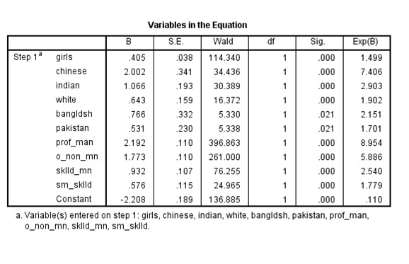
Duplicating the Connelly (2006) Model Results in SPSS
A close look at the results of the model in R indicate that whilst the values of the parameter estimates "estimates" are the same as B in Table 5 (p.20) the standard errors are not the same.
My intuition is that the original analysis was undertaken in SPSS.
This is an unforeseen obstacle.
My desire is to investigate this a little further.
Unfortunately, at the current time there is not a SPSS kernel available within the Jupyter notebook.
However, I have a cunning plan.
First, I will write out the dataset in SPSS format.
write.foreign doesn't generate native SPSS datafiles (.sav) but it does generate is the data in a comma delimited format (a .txt file) and a basic syntax file for reading that data into SPSS (a .sps file).
Using the following general syntax
write.foreign(as.data.frame(mydata), "c:/mydata.txt", "c:/mydata.sps", package="SPSS")
I plan to estimate the logit model in SPSS (with the data weighted).
write.foreign(as.data.frame(mydata4.df), "C:/Users/Vernon/OneDrive - University of Edinburgh/Documents/ycs_9_2017/ycs9sw1_v2.txt", "C:/Users/Vernon/OneDrive - University of Edinburgh/Documents/ycs_9_2017/ycs9sw1_v2.sps", package="SPSS")
Here we leave the Jupyter notebook
We have had to break the workflow because SPSS cannot currently be run in the language agnostic environment of the Jupyter notebook.
To assist with transparency this link shows the model being estimated in SPSS
(IBM SPSS Version 22 Release 22.0.0.1 64-bit)
I am grateful to Dr Roxanne Connelly, University of Warwick, UK (http://www2.warwick.ac.uk/fac/soc/sociology/staff/connelly/) for this suggestion.
I use the following on-line software to record the SPSS job https://www.apowersoft.com/free-online-screen-recorder .
Here is the SPSS syntax that was generated by the write.foreign command.
DATA LIST FILE= "C:/Users/Vernon/OneDrive - University of Edinburgh/Documents/ycs_9_2017/ycs9sw1_v2.txt" free (",") / serial weight sex s1a_c a58 s1eth s1acqe pseg prof_man o_non_mn sklld_mn sm_sklld pseg5 pseg6 pseg7 s15a_c girls ethnic1 white black indian pakistan bangldsh chinese other .
VARIABLE LABELS serial "serial" weight "weight" sex "sex" s1a_c "s1a_c" a58 "a58" s1eth "s1eth" s1acqe "s1acqe" pseg "pseg" prof_man "prof_man" o_non_mn "o_non_man" sklld_mn "skilled_man" sm_sklld "semi_skilled" pseg5 "pseg5" pseg6 "pseg6" pseg7 "pseg7" s15a_c "s15a_c" girls "girls" ethnic1 "ethnic1" white "white" black "black" indian "indian" pakistan "pakistani" bangldsh "bangladeshi" chinese "chinese" other "other" .
VALUE LABELS / sex 1 "not answered (9)" 2 "item not applicable" 3 "male" 4 "female" / a58 1 "not answered (99)" 2 "don't know (98)" 3 "item not applicable" 4 "white" 5 "carib." 6 "afro." 7 "other black" 8 "indian" 9 "pakistani" 10 "bangladeshi" 11 "chin!ese" 12 "other asian" 13 "any other" 14 "mixed ethnic origin" 15 "ref!used" / s1eth 1 "not answered (9)" 2 "schedule not obtained" 3 "schedule not applicable" 4 "item not applicable" 5 "white" 6 "black groups" 7 "asian groups" 8 "mixed/!other groups" 9 "refused/ns" / s1acqe 1 "not answered (9)" 2 "schedule not obtained" 3 "schedule not applicable" 4 "item not applicable" 5 "5+ gcses at a-c" 6 "1-4 gcses at a-c" 7 "5+ gcses at d-g" 8 "1-4 gcses at d-g" 9 "none reported" . EXECUTE.
Here is the SPSS syntax that weights the data and then estimates the logit model.
WEIGHT BY weight.
LOGISTIC REGRESSION VARIABLES s15a_c /METHOD=ENTER girls chinese indian white bangldsh pakistan prof_man o_non_mn sklld_mn sm_sklld /CRITERIA=PIN(.05) POUT(.10) ITERATE(20) CUT(.5).
These results are now the same as in the published model
Complex Samples Logistic Regression.
As a final check I undertake the analysis in SPSS using the Comples Samples approach.
The code required for the complex sample analysis plans is
CSPLAN ANALYSIS
/PLAN FILE='C:\Users\Vernon\OneDrive - University of Edinburgh\Documents\ycs_9_2017\logit.csaplan'
/PLANVARS ANALYSISWEIGHT=weight
/SRSESTIMATOR TYPE=WOR
/PRINT PLAN
/DESIGN
/ESTIMATOR TYPE=WR.
The code required for the complex sample logistic regression model is
CSLOGISTIC s15a_c(LOW) WITH girls chinese indian white pakistan bangldsh prof_man o_non_mn
sklld_mn sm_sklld
/PLAN FILE='C:\Users\Vernon\OneDrive - University of '+
'Edinburgh\Documents\ycs_9_2017\logit.csaplan'
/MODEL girls chinese indian white bangldsh pakistan prof_man o_non_mn sklld_mn sm_sklld
/INTERCEPT INCLUDE=YES SHOW=YES
/STATISTICS PARAMETER SE
/TEST TYPE=F PADJUST=LSD
/MISSING CLASSMISSING=EXCLUDE
/CRITERIA MXITER=100 MXSTEP=5 PCONVERGE=[1e-006 RELATIVE] LCONVERGE=[0] CHKSEP=20 CILEVEL=95
/PRINT SUMMARY CLASSTABLE VARIABLEINFO SAMPLEINFO.
Here is a screen shot of the SPSS output.
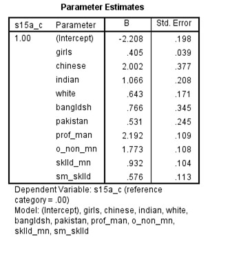
There results are the same as the results in R
It is worth noting that there are (at least) two ways of estimating a logit model in SPSS in the presence of survey weights.
The __Complex Samples__ approach returns the same results as __svy__ in _R_.
By contrast weighting the dataset first, and then estimating a standard logistic regression model leads to different standard errors.
Detective work was required to arrive at this conclusion.
This passage of work underlines the requirement to clearly state the software used (including versions, libraries and dependencies) and as much detail as possible relating to the technique used.
Duplicating the Connolly (2006) Model Results in Stata
In this section I duplicate the results produced in Connolly 2006 using Stata.
We have had to move outside of the workflow in Jupyter (to move to SPSS).
Just in case we should make certain that we have the correct dataset in the frame.
load ("C:/Users/Vernon/OneDrive - University of Edinburgh/Documents/ycs_9_2017/ycs9sw1_v2.rda")
ls()
I will now export data frame to Stata format using the foreign library.
library(foreign)
write.dta(mydata4.df, "C:/Users/Vernon/OneDrive - University of Edinburgh/Documents/ycs_9_2017/ycs9sw1_v2.dta")
You MUST have Stata on your machine!
This section uses ipystata to run Stata via Jupyter magic
see
http://dev-ii-seminar.readthedocs.io/en/latest/notebooks/Stata_in_jupyter.html .
You can install IPyStata 0.3.0 using the following syntax
pip install ipystata
at your command line prompt i.e. c:\Users\Vernon .
This facility is provided here
https://github.com/TiesdeKok/ipystata
The author is Ties de Kok
e-mail: t.c.j.dekok@tilburguniversity.edu
Twitter: @TiesdeKok
You MUST have Stata on your machine!
This cell below imports ipystata so that we can run Stata within this notebook.
import ipystata
If you have an error that looks a bit like this
Error in parse(text = x, srcfile = src): 1:8: unexpected symbol
1: import ipystata
Then you may probably have changed kernel
You MUST CHANGE the Jupyter kernel to PYTHON using the drop down menu Kernel above.
We are now working in Python using Stata via magic cells!
%%stata -o mydata4.df
codebook, compact
%%stata -o mydata4.df
svyset [pweight=weight]
* you may need to set the line size to stop the table going wonky *
set linesize 100
svy:logit s15a_c girls chinese indian white pakistani bangladeshi prof_man o_non_man skilled_man semi_skilled
Here are the result from R
Survey design: svydesign(id = ~serial, data = mydata4.df, weight = ~weight)
| variable | Estimate | Std. Error | t value | Pr |
|---|---|---|---|---|
| (Intercept) | -2.20829 | 0.19802 | -11.152 | < 2e-16 |
| girls | 0.40456 | 0.03926 | 10.305 | < 2e-16 |
| chinese | 2.00231 | 0.37734 | 5.306 | 1.14e-07 |
| indian | 1.06584 | 0.20829 | 5.117 | 3.15e-07 |
| white | 0.64314 | 0.17118 | 3.757 | 0.000173 |
| bangladeshi | 0.76616 | 0.34486 | 2.222 | 0.026323 |
| pakistani | 0.53136 | 0.24503 | 2.169 | 0.030135 |
| prof_man | 2.19209 | 0.10863 | 20.179 | < 2e-16 |
| o_non_man | 1.77251 | 0.10793 | 16.423 | < 2e-16 |
| skilled_man | 0.93217 | 0.10411 | 8.954 | < 2e-16 |
| semi_skilled | 0.57587 | 0.11264 | 5.112 | 3.23e-07 |
Both their coefficients and the standard errors are the same in __ _R_ __ and in __Stata__
In this section I plan to export the data frame "mydata4.df" which is in the file "ycs9sw1_v2" into an Excel format file ".xlsx".
This required the package 'xlsx' to be installed in R .
install.packages('xlsx')
When I first tried this there was an error because a more up to date version of Java is required.
# if the work recommences with this section then the following libraries might be required.
library(foreign)
library(survey)
library(car)
library(dplyr)
library(weights)
library(dummies)
# this library is required.
library(xlsx)
load ("C:/Users/Vernon/OneDrive - University of Edinburgh/Documents/ycs_9_2017/ycs9sw1_v2.rda")
ls()
write.xlsx(mydata4.df, "C:/Users/Vernon/OneDrive - University of Edinburgh/Documents/ycs_9_2017/ycs9sw1_v2.xlsx")
A file called "ycs9sw1_v2.xlsx" has now been written from within R.
Duplicating the Connolly (2006) Model Results in Python
In this section I will attempt to duplicate the logit model Table 5 p.20 Connolly (2006) in Python.
First we have to "import" a package called "pandas".
Pandas is a software library written for the Python programming language for data manipulation and analysis.
import pandas as pd
If you have an error that looks a bit like this
Error in parse(text = x, srcfile = src):
Then you may probably have changed kernel
You MUST CHANGE the Jupyter kernel to PYTHON using the drop down menu Kernel above
Using "read_excel" which is part of pandas which I have already loaded into "pd", I now construct the data frame "df" reading in the data from the Excel (xlsx) file.
df = pd.read_excel("C:/Users/Vernon/OneDrive - University of Edinburgh/Documents/ycs_9_2017/ycs9sw1_v2.xlsx")
df.head()
Python is more general purpose and not primarily orientated towards social science data analysis. Therefore some things are a little more fiddly.
For example before estimating the logistic regression models we must set a constant for all case (int=1).
df['Int']=1
Examining the data in the data frame "df".
df.head()
df.describe()
import statsmodels.api as sm
list(df)
independentVar = ['girls', 'chinese', 'indian', 'white', 'bangladeshi', 'pakistani', 'prof_man','o_non_man','skilled_man','semi_skilled', 'Int']
logReg = sm.Logit(df['s15a_c'] , df[independentVar])
answer = logReg.fit()
answer.summary()
from patsy import dmatrices
y, x = dmatrices('s15a_c ~ 1 + girls + chinese + indian + white + bangladeshi + pakistani + prof_man + o_non_man + skilled_man + semi_skilled' , df)
sm.GLM(endog=y, exog=x, family=sm.families.Binomial(), data_weights=df['weight']).fit().summary()
Beware!
These results do not appear to have been weighted.
# Here is another attempt...

logmodel=sm.GLM(endog=y, exog=x, family=sm.families.Binomial(sm.families.links.logit)).fit()
#sm.GLM(, family=sm.families.Binomial(), data_weights=df['weight']).fit().summary()
logmodel.summary()
Beware!
These results do not appear to have been weighted.
#Here is a third attempt ...

weight =df['weight']
logmodel2=sm.GLM(endog=y, exog=x, sample_weight =weight, family=sm.families.Binomial(sm.families.links.logit)).fit()

#sm.GLM(, family=sm.families.Binomial(), data_weights=df['weight']).fit().summary()
logmodel2.summary()
Beware!
These results do not appear to have been weighted.
In order to investigate this further I will return to R .
Change the kernel back to R .
library(foreign)
library(survey)
library(car)
library(dplyr)
library(weights)
library(dummies)
library(xlsx)
load("C:/Users/Vernon/OneDrive - University of Edinburgh/Documents/ycs_9_2017/ycs9sw1_v2.rda")
ls()
summary(mydata4.df)
In order to check the results produced using Python I will re-estimate the model in R but this time ignoring the sample weights.
modelnw<-glm (s15a_c ~ girls + chinese + indian +
                 white + bangladeshi + pakistani +
                 pakistani + prof_man + o_non_man +
                 skilled_man + semi_skilled, data = mydata4.df, family = "binomial")
summary(modelnw)
These un-weighted results are the same as the Python results.
The weighting in not working in in Python.
Further investigation of how to incorporate survey weights into a logistic regression model using Python is required.
Replicating the Connolly (2006) Model Results with Quasi-Variance
In this section, following the duplication of the logistic rgression results in Table 3 (p.20) of Connolley (2006) I now undertake a replication activity.
In brief, I have concerns about the parameterisation of the ethnicity measure in the logistic regression model.
The reference category is 'Black' pupils.
This is a small category (n=180).
My suspicion is that this is a sub-optimal reference category.
I will investigate the relationship between the categories of ethnicity by estimating quasi-variance based comparison intervals.
An extensive and reproducible introduction is provided by Gayle and Lambert (2007).
The use of quasi-variance based comparison intervals allows a more subtle investigation of the differences between ethnic groups.
The procedure that will be used is described in Firth and De Menezes (2004) an implemented in the R library 'qvcalc'.
To run this procedure you must have __qvcalc__ installed in _R_.
code required in R
install.packages('qvcalc')
Warning.
Within this Jupyter notebook there has been a lot of non-routine work. For example I have 'swivel-chaired' between data analytical software packages and changed kernels.
It may from time to time be necessary to re-start the notebook depending on how stable your computing environment is.
In this section I re-start a R session.
library(foreign)
library(survey)
library(car)
library(dplyr)
library(weights)
library(dummies)

library(MASS)
library(qvcalc)
Various WARNINGS will appear. Don't panic.
I re-load the R file "ycs9sw1_v2.rda".
load("C:/Users/Vernon/OneDrive - University of Edinburgh/Documents/ycs_9_2017/ycs9sw1_v2.rda")
ls()
The data frame is "mydata4.df".
Please double check that an earlier version has not bee loaded!
summary(mydata4.df)
I now re-estimate the logit model that "duplicated" the results in Table 3 (p.20) Connolly (2016).
mydesign2 <- svydesign(id = ~serial,data = mydata4.df, weight = ~weight)
model2<-svyglm (s15a_c ~ girls + chinese + indian +
                 white + bangladeshi + pakistani +
                 pakistani + prof_man + o_non_man +
                 skilled_man + semi_skilled, design=mydesign2, data = mydata4.df, family = "binomial")
summary(model2)
Here is a reminder of the variables that are in the data frame "mydata4.df".
str(mydata4.df)
In order to use the QV procedure I have to estimate the model with a multiple-categorie measure of "ethnicity".
The variable "ethnicity1" has already been created.
I check that "ethnicity1" is a factor.
levels(mydata4.df$ethnic1)
The variable "ethnic1" is not a factor so I am going to declare as a factor.
mydata4.df$ethnic1 <- factor(mydata4.df$ethnic1 )
levels(mydata4.df$ethnic1)
is.factor(mydata4.df$ethnic1)
The variable "ethnic1" is now a factor.
Here I remind myself of the variables in the data frame "mydata4.df" and check again that "ethnic1" is a factor in the dataset.
str(mydata4.df)
ls()
model3<-svyglm (s15a_c ~ factor(ethnic1) + girls + prof_man + o_non_man +
                 skilled_man + semi_skilled, design=mydesign2, data = mydata4.df, family = "binomial")
summary(model3)
BEWARE
The variable "ethnic1" is coded to match the ethnicity measure in Table 1 (p.7) Connolly (2006). However, the order of the dummy variables included in the logistic regression model in Table 3 (p.20) Connelly (2006) do not match.
This could not have easily been foreseen.
In the spirit of showing all of the workflow I have preseved this snippet of data wrangling.
A re-coded version of "ethnic1" is required.
Here is the original variable.
table(mydata4.df$ethnic1)
The new variable will be called "ethnic2".
The reference category should be 'black' pupils (i.e. carib; afro.; other black).
Categories should be
- Black
- Chinese
- Indian
- White
- Bangladeshi
- Pakistani
- Others (but this category has been omitted from the analysis)
# create the new field,

mydata4.df$ethnic2 <- 7

# everyone is placed into category 7.

# recode the new field with values from the old field.
mydata4.df$ethnic2[mydata4.df$a58=="white"] <-4
mydata4.df$ethnic2[mydata4.df$a58=="carib."] <-1
mydata4.df$ethnic2[mydata4.df$a58=="afro."] <-1
mydata4.df$ethnic2[mydata4.df$a58=="other black"] <-1
mydata4.df$ethnic2[mydata4.df$a58=="indian"] <-3
mydata4.df$ethnic2[mydata4.df$a58=="pakistani"] <-6
mydata4.df$ethnic2[mydata4.df$a58=="bangladeshi"] <-5
mydata4.df$ethnic2[mydata4.df$a58=="chin!ese"] <-2
mydata4.df$ethnic2[mydata4.df$a58=="other asian"] <-7
mydata4.df$ethnic2[mydata4.df$a58=="any other"] <-7
mydata4.df$ethnic2[mydata4.df$a58=="mixed ethnic origin"] <-7
mydata4.df$ethnic2[mydata4.df$a58=="ref!used"] <-7
table(mydata4.df$ethnic2)
Just to check the old variable "ethnic1" and the new variable "ethnic2".
mytable <- table (mydata4.df$ethnic1,mydata4.df$ethnic2)
mytable # print table
I will now try to re-estimate the model but with the ethnicity variable "ethnic2".
The data have been altered so I re-set the survey design.
mydesign3 <- svydesign(id = ~serial,data = mydata4.df, weight = ~weight)
model4<-svyglm (s15a_c ~ factor(ethnic2) + girls + prof_man + o_non_man +
                 skilled_man + semi_skilled, design=mydesign3, data = mydata4.df, family = "binomial")
summary(model4)
I now past the modelling results to the quasi-variance estimation package.
model4.qvs <- qvcalc(model4, "factor(ethnic2)")
I now get a summary of these results.
This includes the
parameter estimate (i.e. beta) "estimate";
conventional standard error "SE";
quasi-variance based standard error "quasiSE";
quasi-varianve based variance "quasiVar".
summary(model4.qvs, digits = 4)
I now plot the estimates for "ethnicity2" along with quasi-variance based 95% comparison intervals.
plot(model4.qvs)
The levels for factor(ethnic2)
1 Black; 2 Chinese; 3 Indian; 4 White; 5 Bangladeshi; 6 Pakistani.
Comments
My suspicion that the 'Black' pupils category is a sub-optimal reference category is confirmed.
This is a small category (n=180), and there is a large comparison interval around this estimate.
Also, whilst the other five ethnic categories are significantly different to zero (when Black pupils are set as the reference category) the differences between some categories are not significant. For a fuller discussion of using quasi-variance comparison intervals see Gayle and Lambert 2007.
I will now re-estimate the model with 'White' pupils as the referene category.
I will re-organise the ethnic categories as follows
'White'
'Chinese'
Then the three South Asian categories
'Indian'
'Banglasdeshi'
'Pakistani'
Then finally...
'Black'
(Others are absent from the model)
Re-ordering the ethnicity variable "ethnic2".
Creating a new ethnicity variable "ethnic3".
# create the new field,

mydata4.df$ethnic3 <- 7

# everyone is placed into category 7.

# recode the new field with values from the old field.
mydata4.df$ethnic3[mydata4.df$a58=="white"] <-1
mydata4.df$ethnic3[mydata4.df$a58=="carib."] <-6
mydata4.df$ethnic3[mydata4.df$a58=="afro."] <-6
mydata4.df$ethnic3[mydata4.df$a58=="other black"] <-6
mydata4.df$ethnic3[mydata4.df$a58=="indian"] <-3
mydata4.df$ethnic3[mydata4.df$a58=="pakistani"] <-5
mydata4.df$ethnic3[mydata4.df$a58=="bangladeshi"] <-4
mydata4.df$ethnic3[mydata4.df$a58=="chin!ese"] <-2
mydata4.df$ethnic3[mydata4.df$a58=="other asian"] <-7
mydata4.df$ethnic3[mydata4.df$a58=="any other"] <-7
mydata4.df$ethnic3[mydata4.df$a58=="mixed ethnic origin"] <-7
mydata4.df$ethnic3[mydata4.df$a58=="ref!used"] <-7
table(mydata4.df$ethnic3)
Just to check the old variable "ethnic1" and the new variable "ethnic3".
mytable <- table (mydata4.df$ethnic1,mydata4.df$ethnic3)
mytable # print table
This looks satisfactory.
I will now try to re-estimate the model but with the ethnicity variable "ethnic2".
The data have been altered so I re-set the survey design.
mydesign4 <- svydesign(id = ~serial,data = mydata4.df, weight = ~weight)
model5<-svyglm (s15a_c ~ factor(ethnic3) + girls + prof_man + o_non_man +
                 skilled_man + semi_skilled, design=mydesign4, data = mydata4.df, family = "binomial")
summary(model5)
Note!
The results no longer duplicate Table 5 (p.20) Connolley (2006) but the results build upon, and extend, the work so they are a replication.
I now pass the results to the quasi-variance procedure.
model5.qvs <- qvcalc(model5, "factor(ethnic3)")
summary(model5.qvs, digits = 4)
I now plot the results for "ethnicity3" along with quasi-variance based 95% comparison intervals.
plot(model5.qvs)
The levels for factor(ethnic3)
- White
- Chinese
- Indian
- Banglasdeshi
- Pakistani
- Black
(Others are absent from the model)
Comments
The results have been duplicated and then built upon. These results are a replication.
The model is improved by using 'White' pupils as the reference category. This is a large category and there is a small comparison interval around the estimate.
The model also tells a more theoretically useful substantive story. The use of quasi-variance based comparison intervals allows a more subtle investigation of the differences between ethnic groups.
There are some ethnic differences in school GCSE outcomes (5+ GCSEs at grades A - C).
Compared with the majority of pupils who are white those who are Chinese have better outcomes.
Indian pupils perform better than white pupils.
Bangladeshi and Pakistani pupils do have significantly different outcomes to white pupils.
Black pupils have significantly poorer outcomes than their white counterparts.
It is notable that the three south Asian ethnic groups are not significantly different to each other.
This hopefully illustrates that this model is better parameterised that the original model presented in Table 5 (p.20) Connolly (2006).
The analyses above have required some more data wrangling. Therefore it is prudent to save a new copy of the data.
I will take a look at the objects that are knocking around.
ls()
To avoid confusion later and to help to keep the workflow clear I will create a new data frame "mydata5.df".
mydata5.df<-mydata4.df
str(mydata5.df)
save(mydata5.df,file="C:/Users/Vernon/OneDrive - University of Edinburgh/Documents/ycs_9_2017/ycs9sw1_v3.rda")
Here I make a Stata copy of the file just in case I required it for swivel chair activities later in the workflow.
write.dta(mydata5.df, "C:/Users/Vernon/OneDrive - University of Edinburgh/Documents/ycs_9_2017/ycs9sw1_v3.dta")
Replicating the Connolly (2006) Model Results Adding an Improved Social Class Measure (UK National Socio-economic Classification - NS-SEC)
In this next stage of the analysis I will explore importing an additions social class measure.
The measure of social class that is employed in Table 5 (p.20) Connelly (2006) is unconventional in social stratification research.
The National Socio-economic Classification (NS-SEC) is a commonly used measure in stratification research and is the measure used in official statistics and government research in the United Kingdom.
In the next stage of the analysis I replicate the analysis of school GCSE attainment using YCS Cohort 9 through the incorporation of a parental NS-SEC measure that was derrived by Croxford et al (2007).
Youth Cohort Time Series for England, Wales and Scotland, 1984-2002 UK Data Archive Study 5765
https://discover.ukdataservice.ac.uk/catalogue/?sn=5765
The Education and Youth Transitions project (EYT) was funded by the ESRC from 2003 to 2006.
A key part of the project was to create comparable time-series datasets for England,
Wales and Scotland from the Youth Cohort Study (YCS) and Scottish School Leavers Survey
(SSLS).
Downloaded: UK Data Service https://www.ukdataservice.ac.uk/
Date: 23rd June 2017
Time: 00:17
Croxford, L., Iannelli, C., Shapira, M. (2007). Youth Cohort Time Series for England, Wales and Scotland, 1984-2002. [data collection]. National Centre for Social Research, Scottish Centre for Social Research, University of Edinburgh. Centre for Educational Sociology, [original data producer(s)]. UK Data Service. SN: 5765, http://doi.org/10.5255/UKDA-SN-5765-1
Warning.
Within this Jupyter notebook there has been a lot of non-routine work. For example I have 'swivel-chaired' between data analytical software packages and changed kernels.
It may from time to time be necessary to re-start the notebook depending on how stable your computing environment is.
In this section I re-start a R session.
library(foreign)
library(survey)
library(car)
library(dplyr)
library(weights)
library(dummies)

library(MASS)
library(qvcalc)
Various WARNINGS will appear. Don't panic.
From the Youth Cohort Time Series for England, Wales and Scotland, 1984-2002 UK Data Archive Study 5765, I will import a file called "ew_core". This is the core file containing pupils in England and Wales.
# This file is located on (my) OneDrive.

mydataew.df <- read.dta("C:/Users/Vernon/OneDrive - University of Edinburgh/Documents/ycs_9_2017/ew_core.dta")
summary(mydataew.df)
To see the summary of the data use the scroll bar to scroll down.
str(mydataew.df)
The variables that I require are
t0cohort - the YCS cohort (i.e. year).
t0nation - identifies if the pupil is from the England and Wales data (this is just a check the dataset should be England and Wales on hence "ew" in "ew_core.dta" .
t0caseid - this is an id variable. However, it is not unqiue across YCS cohorts so must be used in conjuction with a cohort identifier.
t0source - identifies the YCS cohort (e.g. YCS 9).
t1weight - this is the sweep 1 survey weight.
t1resp - identifies if the pupil responded in sweep 1 of the survey.
t0parsec - this is the parental NS-SEC measure (8 category) that is derrived by Croxford et al. (2007). This is the measure that I require for the current replication exercise.
table(mydataew.df$t0cohort)
table(mydataew.df$t0source)
table(mydataew.df$t0parsec)
Get a subset of the data with only the variables needed.
myvarsew <- c("t0cohort", "t0nation", "t0caseid", "t0source", "t1weight", "t1resp", "t0parsec")
mydataew.df <- mydataew.df[myvarsew]
summary(mydataew.df)
Now I get a subset of the cases (i.e. pupils) that are in the YCS cohort 9.
mydataew2.df <- mydataew.df[ which(mydataew.df$t0source=="ycs9"),]
summary(mydataew2.df)
table(mydataew2.df$t0source)
I will now check which objects are knocking around.
ls()
I will now (re-)load the last version of my YCS cohort 9 dataset "ycs9sw1_v3.rda".
load("C:/Users/Vernon/OneDrive - University of Edinburgh/Documents/ycs_9_2017/ycs9sw1_v3.rda")
ls()
str(mydata5.df)
This data frame should have "ethnic2" and "ethnic3" in it.
If they are absent then a older file has been used.
I am now going to wrangle the data a little.
The reshape library is required if it is not already loaded.
library(reshape)
The 'id" variables in file "ew_core" (i.e. Croxford's time series files) is not the same as in YCS cohort 9 file "ycs9sw1".
Therefore I am going to change the variable "t0caseid" which is in "ew_core" to "serial" which is the name of the "id" variable in "ycs9sw1".
mydataew2.df <- rename(mydataew2.df, c(t0caseid="serial"))
str(mydataew2.df)
Now I combine the file "ycs9sw1_v3" which is in data frame mydata5.df with "ew_core" which is in data frame mydataew2.df.
mydata6.df <- merge(mydata5.df, mydataew2.df,by="serial")
str(mydata6.df)
If this has worked then mydata6.df should contain "ethnic2", "ethnic3" and "t0parsec".
Here is the first glimpse at the parental NS-SEC variable "t0parsec".
mytablenssec <- table(mydata6.df$t0parsec, mydata6.df$s15a_c)
mytablenssec # print table
prop.table (mytablenssec, 1)
save(mydata6.df,file="C:/Users/Vernon/OneDrive - University of Edinburgh/Documents/ycs_9_2017/ycs9sw1_v4.rda")
load ("C:/Users/Vernon/OneDrive - University of Edinburgh/Documents/ycs_9_2017/ycs9sw1_v4.rda")
ls()
Takin a second look at NS-SEC the social class variable.
mytablenssec <- table(mydata6.df$t0parsec, mydata6.df$s15a_c)
mytablenssec # print table
There is a missing value coded as "99".
mydata6.df$t0parsec[mydata6.df$t0parsec=="99"] <-NA
mytablenssec <- table(mydata6.df$t0parsec, mydata6.df$s15a_c)
mytablenssec # print table
I now check that "t0parsec1" is a factor.
levels(mydata6.df$t0parsec )
The variable "t0parsec" is not a factor so I am going to declare as a factor.
mydata6.df$t0parsec <- factor(mydata6.df$t0parsec )
levels(mydata6.df$t0parsec)
is.factor(mydata6.df$t0parsec)
I now estimate a logit model of school GCSE outcomes (5+ GCSEs and grade A - C).
It will be a survey based model (svy).
Outcome variable "s15a_c".
Explanatory variables "girls", "ethnic3", "t0parsec".
mydesign5 <- svydesign(id = ~serial,data = mydata6.df, weight = ~weight)
model6<-svyglm (s15a_c ~ girls + factor(ethnic3) + factor(t0parsec), design=mydesign5, data = mydata5.df, family = "binomial")
summary(model6)
I now pass the results to the quasi-variance procedure.
model6.qvs <- qvcalc(model6, "factor(t0parsec)")
summary(model6.qvs, digits = 4)
I now plot the results for "t0parsec" along with quasi-variance based 95% comparison intervals.
plot(model6.qvs)
Parental Social Class NS-SEC (t0parsec)
1.1 Large employers and higher managerial and administrative occupations
1.2 Higher professional occupations
2 Lower managerial, administrative and professional occupations
3 Intermediate occupations
4 Small employers and own account workers
5 Lower supervisory and technical occupations
6 Semi-routine occupations
7 Routine occupations
8 Never worked and long-term unemployed
Comments
The National Socio-economic Classification (NS-SEC) is a commonly used measure in stratification research and is the measure used in official statistics and government research in the United Kingdom. In this model I replicated the analysis of school GCSE attainment using YCS Cohort 9 through the incorporation of a parental NS-SEC measure that was derrived by Croxford et al (2007).
The analyses above have required some more data wrangling. Therefore it is prudent to save a new copy of the data.
I will take a look at the objects that are knocking around.
ls()
To avoid confusion later and to help to keep the workflow clear I will create a new data frame "mydata6.df".
mydata6.df is a file that combines YCS cohort 9 file "ycs9sw1" [SN: 4009] and "ew_core" from Croxford (2007) [SN: 5765].
str(mydata6.df)
save(mydata6.df,file="C:/Users/Vernon/OneDrive - University of Edinburgh/Documents/ycs_9_2017/ycs9sw1_v4.rda")
Here I make a Stata copy of the file just in case I required it for swivel chair activities later in the workflow.
write.dta(mydata6.df, "C:/Users/Vernon/OneDrive - University of Edinburgh/Documents/ycs_9_2017/ycs9sw1_v4.dta")
Producing a Data Dictionary (or Codebook)
load ("C:/Users/Vernon/OneDrive - University of Edinburgh/Documents/ycs_9_2017/ycs9sw1_v4.rda")
ls()
str(mydata6.df)
myvarscb <- c("serial", "weight", "s15a_c", "girls", "ethnic1", "ethnic2", "ethnic3",
"white", "black", "indian", "pakistani", "bangladeshi", "chinese", "other",
"prof_man", "o_non_man", "skilled_man", "semi_skilled", "t0parsec")
mydata7.df <- mydata6.df[myvarscb]
str(mydata7.df)
Data Dictionary (or Codebook)
This is the codebook for the file ycs9sw1_v4.rda which contains mydata6.df .
serial id variable unique to YCS cohort 9
weight survey weight sweep 1 YCS cohort 9
s15a_c outcome variable 5+ GCSEs A (star) - C constructed from variable "s1a_c"
0 = 1 - 4 GCSEs grades A (star) - C
1 = 5+ GCSEs grades A (star) - C
girls gender variable constucted from variable "sex"
0 = boys
1 = girls
ethnic1 ethnicity variable constructed from variable "a58"
1 White
2 Black
3 Indian
4 Pakistani
5 Bangladeshi
6 Chinese
7 Other (but this category has been omitted from the analysis because it is omitted in Connolly 2006)
ethnic2 ethnicity variable constructed from variable "a58"
1 Black
2 Chinese
3 Indian
4 White
5 Bangladeshi
6 Pakistani
7 Others (but this category has been omitted from the analysis because it is omitted in Connolly 2006)
The variable ethnic1 is coded to match the ethnicity measure in Table 1 (p.7) Connolly (2006). However, the order of the dummy variables included in the logistic regression model in Table 3 (p.20) Connelly (2006) do not match. The reference category for the logistic regression should be 'black' pupils (i.e. carib; afro.; other black). This could not have easily been foreseen.
ethnic3 ethnicity variable constructed from variable "a58"
This variable is used in the "replication" model.
The majority group 'white' pupils are now the reference category.
The three south Asian categories are adjacent to each other.
1 'White'
2 'Chinese'
3 'Indian'
4 'Banglasdeshi'
5 'Pakistani'
6 'Black'
(Others are absent from the model)
white dummy variable constructed from variable "ethnic1"
0 = non-white
1 = white
black dummy variable constructed from variable "ethnic1"
0 = non-white
1 = white
indian dummy variable constructed from variable "ethnic1"
0 = non-white
1 = white
pakistani dummy variable constructed from variable "ethnic1"
0 = non-white
1 = white
bangladeshi dummy variable constructed from variable "ethnic1"
0 = non-white
1 = white
chinese dummy variable constructed from variable "ethnic1"
0 = non-white
1 = white
other dummy variable constructed from variable "ethnic1"
0 = non-white
1 = white
prof_man dummy variable parents in professional / managerial social class constructed from variable "pseg1"
0 = no
1 = yes
o_non_man dummy variable parents in other non-manual social class constructed from variable "pseg2"
0 = no
1 = yes
skilled_man dummy variable parents in skilled-manual social class constructed from variable "pseg3"
0 = no
1 = yes
semi_skilled dummy variable parents in semi-skilled manual social clas constructed from variable "pseg4"
0 = no
1 = yes
t0parsec categorical variable parents social class - a derrived variable Croxford et al. (2007) SN: 5765,
The UK National Socio-economic Classification (NS-SEC) 8 category version
1.1 Large employers and higher managerial and administrative occupations
1.2 Higher professional occupations
2 Lower managerial, administrative and professional occupations
3 Intermediate occupations
4 Small employers and own account workers
5 Lower supervisory and technical occupations
6 Semi-routine occupations
7 Routine occupations
8 Never worked and long-term unemployed
Discussion
The Pre-Analysis Plan Reviewed
In this section I review the pre-analysis plan compare it with the work that was actually produced.
The pre-analysis plan is available here https://github.com/vernongayle/new_rules_of_the_sociological_method/blob/master/pre_analysis_plan_20170624_vg_v1.docx .
Tasks
1). Duplication of Logistic Regression Model Reported in Connolly (2006)
Achieved.
2). Replication of Logistic Regression Model Reported in Connolly (2006) Using Quasi-Variance based Estimation
Achieved.
3). Replication of Logistic Regression Model Reported in Connolly (2006) Adding National Socio-economic Classification (NS-SEC) Measure Social Class from UK Data Archive Study 5765
Achieved.
Deliverables
1). A reproducible workflow within a Jupyter notebook deposited in a Git repository
Achieved.
2). A data dictionary (codebook) accompanying the work
Achieved.
The Reproducibility Checklist Revisited
In this section I reflect on how the work compares with Stark's Reproducibility Checklist.
http://www.bitss.org/2015/12/31/science-is-show-me-not-trust-me/
Philip Stark outlines 14 reproducibility points that an analysis can fail on
1. If you relied on Microsoft Excel for computations
Excel was not used in this work.
2. If you did not script your analysis, including data cleaning and munging
All of the analysis was scripted see Data Wrangling and Data Analysis
3. If you did not document your code so that others can read and understand it
As far as practicable I have attempted to write this Jupyter notebook as a 'literate data analysis document'.
I provided information on using this notebook, and on the authorship and meta-information.
4. If you did not record and report the versions of the software you used (including library dependencies)
I reported on the computing environment and data analysis software including library dependencies.
5. If you did not write tests for your code
I provided two code tests, one for logistic regression and one for quasi-variance estimation, which are checked against published results.
6. If you did not check the code coverage of your tests
I did not write or use any new tests.
7. If you used proprietary software that does not have an open-source equivalent without a really good reason
The data enabling (i.e. wrangling and cleaning) and the analyses were undertaken in R which is an open-source software.
8. If you did not report all the analyses you tried (transformations, tests, selections of variables, models, etc.) before arriving at the one you chose to emphasize
I reported on all the analyses including data transformations, tests, selections of variables, alternative models and failed activities.
9. If you did not make your code (including tests) available
Information on how the code is licensed is provided. The code will be made available using Github https://github.com/vernongayle .
10. If you did not make your data available (and a law like FERPA or HIPPA doesn’t prevent it)
The data cannot be made publically available but researchers can assess the data from the UK Data Service https://www.ukdataservice.ac.uk/ .
11. If you did not record and report the data format
A description of the research dataset and well as information on the data format and the time and date of the dowload are provided (similar information is provided for the Croxford et al. (2007) dataset which is used to harvest an alternative social class measure.
12. If there is no open-source tool for reading data in that format
The code to read the data, wrangle the data and produce all of the results is written in R which is open-source and will be provided in a Jupyter notebook which is also open-source and will be made available using the open-source platform Github https://github.com/vernongayle.
13. If you did not provide an adequate data dictionary
A data dictionary (or codebook) is provided.
14. If you published in a journal with a paywall and no open-access policy
The work has not yet been published. But it will be available through UK green open access policy via my university repository http://www.research.ed.ac.uk/portal/en/persons/vernon-gayle(682d7da1-a2ad-49f0-b36c-64478c658f99).html .
Conclusions
The overall motivation of this work was to explore the practicability of using Stark’s ‘reproducibility check list’ in a piece of sociological research using genuine large-scale social science data.
The work on this project provides a striking reminder of the large amount of data enabling (i.e. data wrangling) that is required to duplicate a relatively straightforward published result. Despite knowing the data resource relatively well, duplicating a logit model with only three explanatory variables took me effort and some detective work. The conclusions that are drawn are the result of what is an early exploration. After further reflection and discussions they are likely to be refined. As they currently stand my conclusions are unlikely to be the last word on the subject of undertaking reproducible social science using large-scale and complex datasets.
In this section I will reflect on the items on Stark’s checklist and comment on their relevance and feasibility for sociological research using large-scale social science datasets.
1. If you relied on Microsoft Excel for computations, fail.
There is little justification for using a spreadsheet to undertake analyses of large-scale social science datasets. It is almost impossible to provide and document a clear audit trail when using a spreadsheet. The now well-known case of the errors in the spreadsheet-based calculations made in Reinhart and Rogoff (2010a; 2010b) which were reported by Herndon, Ash and Pollin (2014) should serve as a stern warning against using spreadsheets in social science data analyses. In addition Stark points to the more general problems of bugs in spreadsheet software (see also http://eusprig.org/horror-stories.htm).
2. If you did not script your analysis, including data cleaning and munging, fail.
Scripting the workflow is integral to successful social science data analysis. Having a planned and organised workflow is indispensable to producing high-quality social science research. Long (2009) provides an authoritative account of good practices in the social science data analysis workflow. More recently these principles have been distilled in Gayle and Lambert (2017).
In practice large-scale social science datasets are almost never delivered in an immediately ‘analysis-ready’ format. The data analyst will almost always have to undertake some activities to enable the data for analysis. I use the term ‘data enabling’ to describe the stage between downloading the social science dataset (for example from a national archive) and beginning to undertake statistical analyses. ‘Data enabling’ comprises tasks associated with preparing and enhancing data for statistical analysis, such as recoding measures, constructing new variables and linking datasets (Blum et al., 2009; Lambert and Gayle, 2008). ‘Data enabling’ is a substantial part of the research process but its importance is often overlooked. The time required to ‘enable data’ is frequently underestimated, even by more experienced social science data analysts.
An audit trail, which acts as a set of breadcrumbs is essential for navigating back through data enabling aspects of the workflow, and is therefore essential for determining the provenance of results. A scripted workflow is essential for accurate, efficient, transparent and reproducible social science research.
3. If you did not document your code so that others can read and understand it, fail.
Documenting research code is central to delivering reproducible work. The concept of making the workflow 'literate' is new within sociological research. The idea of producing explanations of the thinking behind individual steps in the workflow is novel. Producing commentaries in human readable language (e.g. plain English) interwoven between research code and outputs is innovative. The material produced above shows promising signs that this approach will pay dividends in making research endeavours more transparent and therefore reproducible.
I am mindful of the old saying ‘that a recipe is not a recipe until someone else has cooked it’. A thoroughgoing proof of the literacy and the transparency of research code is only achieved when a third party, who is unconnected with the work, has successfully followed and executed the code. As a result of this position I am increasingly advocating activities such as the pair production of research code, and peer reviewing of research code. These activities will represent a marked change in how sociological research using large-scale datasets is routinely undertaken. If these activities are taken-up, and taken seriously, they will have consequences for how research teams undertake work, and how researchers are trained (and re-trained).
4. If you did not record and report the versions of the software you used (including library dependencies), fail.
This is easily achieved, and can prove to be critical later when a researcher is trying to ‘duplicate’ the work (i.e. produce identical results). The exact results reported in table 5 Connolly (2006 p.20) could not immediately be duplicated even though identical variables were constructed. It took some detective work to ascertain that the work was undertake using SPSS in a specific mode. Since many analyses use special libraries and routines it is important that they are precisely documented so that results can be duplicated and ultimately be checked and validated.
5. If you did not write tests for your code, fail.
This is a sensible requirement, however because many sociological analysis employ standard and routine methods it may be too stringent a requirement for every single sociological analysis. In this present analysis I compared the results of two methods, which were then used in the analysis, against existing published results. Stark suggests that you should test your software every time you change it. This is a sensible and reasonable precaution, and when network versions of software are changed or updated, universities and research institutions should re-test their software.
6. If you did not check the code coverage of your tests, fail.
Stark suggests that this would be a good practice but he has never seen a scientific publication that does so. As far as I understand it, in computer science, code coverage is a measure used to describe the degree to which the source code of a program is executed when a particular test suite (a set of cases intended to be used to test a software program to show that it has some specified set of behaviours) runs. In theory a program with high code coverage has had more of its source code executed during the testing which might suggest it has a lower chance of containing undetected errors.
On reflection few sociological researchers develop new statistical tests or need to implement statistical tests within new software routines. Therefore this requirement is probably irrelevant to most mainstream sociological analyses using large-scale datasets. For researchers who are developing new tests or constructing new routines then testing the coverage of their code and clearly documenting it would be a sensible action.
7. If you used proprietary software that does not have an open-source equivalent without a really good reason, fail.
It is unrealistic to undertake anything more than extremely basic analyses of survey data without using data analysis software. The requirement to use non-proprietary software however is likely to prove controversial within the community of sociological researchers using large-scale datasets.
The freeware R provides a viable approach with a substantial volume of analytical options and considerable programming flexibility (Long, 2011). I have shown in this analysis that R can be used in a standard piece of sociological inquiry. The UK Data Service currently provides datasets in SPSS and Stata format. These formats can be read in R. The UK Data Service provides data in a more package agnostic tab-delimited format. Some R users advocate importing data in this format. In my experience this format can prove challenging to work with especially when matching and merging files and undertaking data analysis enabling tasks.
I am a sociologist who has been undertaking research with large-scale and complex datasets for nearly a quarter of a century, and have taught data analysis to undergraduate and post-graduate students, early career researchers and non-academic researchers. In my experience for sociology students the R learning curve is steep. The skills which are necessary to effectively exploit R through textual programming seem unlikely to lead to its universal adaptation amongst the wide ranging user-communities within the social sciences (see Lambert et al., 2015). A limitation is that R is currently not well suited to the analysis of large-scale social surveys. For example when using R it is difficult to effectively combine the numeric codes for variables along with both their value and variable labels. This means that users are not able to effectively exploit the meta-information on measures that is helpful for routine survey data analysis tasks. A current limitation of R is that there is a lack of clear and concise help files which contain applied examples that relate to the analysis of large-scale and complex social science datasets.
Within this research example I have undertaken a small amount of analysis using Python which is an emerging open-source alternative to R. I was unable to undertake a survey weighted analysis using a logistic regression model, but this may in part be due to my lack of competence with this software. A severe limitation of Python is that there is very little help and almost no applied examples that relate to the analysis of large-scale and complex social science datasets. At the current time there are fewer statistical routines and libraries available in Python, and Python does not offer an alternative to many packages that are available in R. Python is a widely used high-level programming language for general purpose programming. Python is emerging as a valuable tool in data science (e.g. for example web scrapping). In future it might unfold as a viable software for the analysis of large-scale social science datasets.
I have generally been an advocate of using Stata for the analysis of large-scale and complex social science datasets (see Gayle and Lambert 2017). Stata stands out as a sensible choice because it is a popular commercial package with a wide community of social science users. The Stata learning curve is less steep and Stata has very good documentation. Within Stata there are a wide range of analytical capabilities, and ongoing developmental activities (see Lambert et al., 2015). I have found that overall it is the single most effective and efficient tool for undertaking and successfully completing survey data analysis. The tasks associated with data enabling, exploratory data analyses, building statistical models and organising presentation-ready and publication-ready outputs (by which we mean high-quality graphs and tables of modelling results), can all be undertaken using Stata in a single uniformed environment. The development of a Stata kernel in Jupyter, and the ability to use Stata via magic cells (as demonstrated above) illustrate how the software can effectively be used within a notebook. This is attractive for developing transparent research and bundling it within a unified research object.
SPSS is a fairly ubiquitous within sociology departments. It is suited to the analysis of large-scale datasets but compared with Stata it is far more restricted in the range of statistical models that it can estimate. SPSS currently has fewer options for estimating models that are appropriate for longitudinal data. Stata is able to offer more comprehensive facilities to analyse survey datasets with complex designs and selection strategies. This is a clear benefit for social scientists working with contemporary datasets such as the UK Household Longitudinal Study (Understanding Society) and the UK Millennium Cohort Study
In practice, given the current research climate within sociology, the programing knowledge and levels of data analysis skill, the requirement to abandon proprietary software is probably too impractical a step. The requirement could be relaxed to using an established mainstream data analysis software (e.g. Stata, SPSS, R or SAS), but the data enabling and the data analysis must be scripted in as ‘literate’ a fashion as possible. This is essential so that a third party who is unconnected with the project can follow and understand the workflow. Where possible it would be a good practice to augment the work by reporting how an open-source analysis could be undertaken in order to assist in the duplicating (and therefore the checking) results. In practice this might mean undertaking the data enabling and analysis in Stata but documenting how the work could also be reproduced in R or Python.
8. If you did not report all the analyses you tried (transformations, tests, selections of variables, models, etc.) before arriving at the one you chose to emphasize, fail.
Providing access to the complete workflow is an indispensable aspect of rendering sociological analysis transparent and reproducible. The use of Jupyter notebooks is a concrete example of organising or bundling the elements of the workflow into a ‘research object’ (see http://www.researchobject.org/). The use of Jupyter notebooks in sociological research extends the possibilities of material being Findable, Accessible, Interoperable and Reusable (FAIR) which is a tenet of reproducible science.
9. If you did not make your code (including tests) available, fail.
Stark states that your code should also state how it is licensed. This is a new departure in sociological research. There are a series of licenses that would be appropriate to this activity and that would chime with the wider academic ideas of attribution. In this present work I have chosen to use the MIT License.
Stark further asserts that code should be published in a way that makes it easy for others to check, re-use and extend, for example by publishing it using services like Git repositories. At the current time very few sociological analyses of large-scale and complex datasets have reported all the code used to enable data and then to undertake the analysis.
Few sociological studies have used repositories. Git repositories are primarily used for source code management in software development, but can be used to keep track of changes in any set of files. These services are sometime referred to as version control software (VCS). Gentzkow and Shapiro (2014) is a rare example of VCS being recommended in the social sciences. Mercurial is an alternative to Git and, whilst GitHub has been used in this example other approaches such as BitBucket provide similar services.
10. If you did not make your data available (and a law like FERPA or HIPPA doesn’t prevent it), fail.
Access to data is an integral part of transparent and reproducible social science research. The accessibility of data presents an obstacle for sociologists working with large-scale datasets. Much of the sociological analysis undertaken using large-scale and complex datasets is secondary analysis of general (or omnibus) data resources. These data resources are often national level surveys (for example the US Panel Study of Income Dynamics or the British Household Panel Survey) or data collected as part of national level Censuses. These data do not ‘belong’ to the data analyst and are usually provided by a national archive or other data provider under some form of ‘end user license’. In practice these data are made available for research but cannot be freely shared, and all users must formally registered for the data. The rules and regulations of data use vary across countries, between data providers, and between datasets. Administrative data resources (e.g. education records) usually have tighter controls placed on their use. Sensitive or confidential data (specially relating to health) are usually especially securely controlled.
Unless the data have been collected by the sociologist, and are owned and controlled by them it is unlikely that they will be able to freely share the data that have been analysed in a particular piece of work. Therefore in order to facilitate transparent and reproducible work sociologists should provide as much information on the dataset (including detailed information on versions and downloads) in order to allow a third party to get access to the data that were genuinely used in the analysis.
11. If you did not record and report the data format, fail.
In order to facilitate transparent and reproducible work sociologists should provide as much information on the dataset (including detailed information on versions and downloads) in order to allow a third party to get access to the data there were genuinely used in the analysis. This is especially important when the data are not freely available and have to be accessed via a national repository or through a data provider (see point 10 above).
12. If there is no open source tool for reading data in that format, fail.
This point is critical when datasets are being made available alongside other research objects. In short, if data are unreadable then they do not add to transparency or reproducibility.
In the case of secondary analysis of existing large-scale dataset that have been provided by national data archives it is important that the code to read the data, to enable the data, and to produce all of the results is written in an accessible way. In this current project I have used R which is open-source and code is provided in a Jupyter notebook which is also open-source, and will be made available using the open-source platform Github https://github.com/vernongayle.
13. If you did not provide an adequate data dictionary, fail.
Providing an adequate data dictionary is a relatively easy task but it is not currently a ubiquitous practice. The acid test of a data dictionary is how easily it can be read, and how useful it is for working with the data for a third party who is unconnected with the project.
14. If you published in a journal with a paywall and no open-access policy, fail.
In the pursuit of transparent and reproducible sociological research having open access to published work is critical.
Stark suggests that posting the final version of your paper on a reprint server might be enough, but he thinks that it is time to move to open scientific publications. He further states that most publishers he has worked with have let him mark up the copyright agreements to keep copyright and grant them a non-exclusive right to publish.
In the context of UK higher education research, the move to Green open access will improve the accessibility of published work. Green open access involves publishing in a traditional subscription journal as usual, but also ‘self-archiving’ in a repository (e.g. a university archive or external subject-based repository) and providing free access (although this might be after an embargo period set by the publisher). The UK Research Council which funds research has a preference for immediate, unrestricted, on‐line access to peer‐reviewed and published research papers, free of any access charge and with maximum opportunities for re‐use. This is commonly referred to as Gold open access (see http://www.rcuk.ac.uk/documents/documents/rcukopenaccesspolicy-pdf/).
In conclusion Stark's Reproducibility Checklist provides an important set of benchmarks, and they can reasonably be regarded as a Berkelium Standard (i.e. beyong gold). The items on the checklist represent solid targets to aim for. Given the present research culture in sociology, the programing skills, and the data analytical capabilities of researchers, the items on Stark's Reproducibility Checklist probably represent too large a step forward at the current time.
Therefore in the next section I posit Some Newer Rules of the Sociological Method which might act as a more immediate and practicable set of guidelines for undertaking reproducible sociological research using large-scale and complex social surveys and administrative datasets.
Some Newer Rules of the Sociological Method
The ultimate goal: The providence of every result should be clear and as open as possible.
The overall aim: There should be enough suitable information available to completely duplicate results, without having to contact the authors.
Here are 5 broad ‘Newer Rules of the Sociological Method’ that are tailored to the analysis of large-scale and complex social science datasets.
Use established data analysis software (e.g. Stata, SPSS, or R), and clearly state the version, libraries, dependencies and plugins.
Clearly identify the version of the dataset and its origins (i.e. where and when it was obtained).
Write down all of the code for how the data were prepared for analysis, in a format that it can easily be read by someone unconnected with the project.
Write down all of the code for all of the analyses undertaken and not just the analyses that are presented, in a format that it can easily be read by someone unconnected with the project.
Archive the material in an accessible format at a reachable location.
Within the archive
a) Provide suitable auxillary information describing the contents of the archive, so that in future a third party unconnected with the project can understand the materials.
b) Provide a detailed codebook.
c) Make available all of the research code and information generated within the workflow.
The archived materials should be openly available. Try to use recognised file formats and think about how best to help a third party who is unconnected with the project understand the contents of the archive at some time in the future.
References
Blum, J.M., Warner, G., Jones, S., Lambert, P., Dawson, A., Tan, K.L.L. and Turner, K.J., 2009. Metadata creation, transformation and discovery for social science data management: The DAMES Project infrastructure. IASSIST Quarterly, 33(1), pp.23-30.
Gayle, V. and Lambert, P., 2017. The Workflow: A Practical Guide to Producing Accurate, Efficient, Transparent and Reproducible Social Survey Data Analysis, Working Paper 1/17 UK National Centre for Research Methods, http://eprints.ncrm.ac.uk/4000/.
Gentzkow, M. and Shapiro, J., 2014. Code and data for the social sciences: A practitioner’s guide, University of Chicago mimeo. Available at: https://web.stanford.edu/gentzkow/research/CodeAndData.pdf (accessed 13th December 2016).
Herndon, T., Ash, M. and Pollin, R., 2014. Does high public debt consistently stifle economic growth? A critique of Reinhart and Rogoff. Cambridge Journal of Economics, 38(2), pp.257-279.
Lambert, P., Browne, W. and Michaelides, D, 2015. Contemporary developments in statistical software for social scientists, in Procter, R. and Halfpenny, P. (eds) Innovations in Digital Research Methods. London: Sage.
Lambert, P. and Gayle, V., 2008. Data management and standardisation: A methodological comment on using results from the UK Research Assessment Exercise 2008, DAMES Project Technical Paper 3.
Long, J.D., 2011. Longitudinal data analysis for the behavioral sciences using R. New York: Sage.
Long, J.S. and Long, J.S., 2009. The workflow of data analysis using Stata. College Station, TX: Stata Press.
Reinhart, C. and Rogoff, K., 2010A. Growth in a Time of Debt, Working Paper no. 15639,
National Bureau of Economic Research, http://www.nber.org/papers/w15639.
Reinhart, C. and Rogoff, K., 2010B. Growth in a Time of Debt, American Economic Review, vol.
100, no. 2, 573–8
Converting this Jupyter Notebook into Portable Formats
see http://nbconvert.readthedocs.io/en/latest/
- At the cmd prompt conda install nbconvert
- Change directory (for example my directory is C:\Users\Vernon
- Type jupyter nbconvert --to html mynotebook.ipynb